Get Better Demand Forecasting With a Hybrid Model

When I started working in the oil and gas industry more than a decade ago, the supply chain was characterized by uncertainty in demand. Field problems were quickly escalated to the factory, with the hope that finished goods would be readily available to address demand in an expeditious manner.

My continuous engagement in resolving this persistent supply chain issue prompted me to seek a better solution. As I explored available statistical and machine learning (ML) techniques, my goal was to identify an approach that would be beneficial in developing (1) a forecasting framework to solve the problem of intermittent demand and (2) enable our manufacturing company to quickly meet the dynamic needs of the energy market.

More advanced ML approaches are essential for managing sporadic and lumpy demand patterns where many periods exhibit zero demand interspersed with irregular, high-volume spikes.

How This Approach Applies to Other Industries

These techniques decompose demand into inter-demand intervals (time between orders) and demand sizes (quantity per order), enabling more accurate predictions than traditional forecasting models, which falter on high zero proportions (often less than 50 percent). Their applicability spans diverse industries due to the ubiquity of intermittent patterns in real-world supply chains, driven by factors like seasonal variability, technological obsolescence and event-based consumption.

By estimating lead times and safety stocks as precisely as possible in manufacturing and spare parts logistics, companies can reduce holding costs by 20 percent to 30 percent while minimizing stockouts that could halt production lines. This can be seen in automotive or aerospace, where parts for consumable components demand changes sporadically during maintenance cycles.

In retail and fashion, where trends lead to bursty sales (like sales blitzes of seasonal apparel or promotional items), these methods integrate with demand sensing to adjust replenishment dynamically. This curbs overstock of slow movers and captures impulse buys, thus boosting margins in fast-paced environments like e-commerce platforms.

Health care benefits immensely from intermittent forecasting for pharmaceuticals and medical devices; rare disease treatments or surgical implants exhibit low-volume, unpredictable orders tied to patient events, allowing hospitals to maintain just-in-time inventories that comply with regulatory shelf-life constraints and cut waste.

The energy sector, including renewables like wind turbine blades, applies it to forecast maintenance-driven demands amid variable weather impacts, ensuring reliability without tying up excess capital. Even in high-tech electronics, component sourcing for gadgets faces intermittency from product lifecycles, where advanced ML variants help mitigate bullwhip effects in global supply chains.

The “why” boils down to economic imperatives: Intermittent demand inflates uncertainty, leading to either excess inventory (tying up capital, risking obsolescence) or shortages (lost sales and reputational damage). These methodologies enhance forecast accuracy by 15 percent to 40 percent over naive benchmarks, fostering resilient operations in volatile markets. As data analytics evolve, hybrid models incorporating external covariates (economic indicators) further amplify their value, making them indispensable for sustainable, customer-centric supply chain strategies across sectors.

A Working Example

Intermittent demand is characterized by periods of zero demand followed by small to large demand spikes. It’s often seen in products like spare parts, seasonal goods, or items nearing the end of their life cycles. This pattern is prevalent in industries beyond oil and gas, including manufacturing, retail, health care, and electronics, where it poses unique challenges for inventory planning and forecasting accuracy.

In traditional forecasting, the most common univariate methods employed are simple moving average, exponential smoothing and autoregressive integrated moving average (ARIMA). With intermittent data, there is an upward bias in the forecast directly after a non-zero demand that leads to poor forecast projections.

Filter cartridges illustrate the intermittent demand problem. One of the most common products used in oil and natural gas filtration, filter cartridges are a critical component in the filtration process. Depending on the impurity content and timing of the movement of liquid or gas through the pipeline, the amount of impurities coming out of the ground is anyone’s guess.

Ensuring the removal of solid and liquid contaminants before the liquid or gas enters transmission pipelines, prior to arrival at the refinery, is essential — and any factory or distributor must maintain optimal inventory levels of these cartridges to avoid process disruptions, while minimizing holding costs.

However, demand forecasting for filter cartridges presents a significant challenge due to their intermittent usage, which — due to the unpredictable nature of the impurities — is characterized by sporadic, lumpy demand, with many zero-demand periods followed by sudden spikes.

Traditional Forecasting Methods

The methods employed for intermittent demand forecasting generally fall into the following three categories: model-based, statistical and ML.

Model-based methods include (1) discrete ARIMA, which extends traditional ARIMA for count data, but struggles with zero-heavy series, and (2) integer-valued auto regressive moving average (INARMA). The latter is designed for count data, but it’s complex to implement and general not included in standard libraries.

There are three types of statistical methods:

• Croston’s method, which separates demand size from interarrival time. It’s commonly used for items that have an average demand interval that is greater than 20.
• Syntetos-Boylan approximation (SBA), which addresses Croston’s positive bias.
• The Teunter-Syntetos-Babai (TSB) model, which updates demand probability estimates dynamically.

ML frameworks for handling intermittency are (1) bootstrapping, which generates synthetic demand patterns for model training and (2) temporal aggregation, which reduces intermittency by aggregating over longer time periods.

While the traditional forecasting methods and ARIMA models offer simplicity and smooth, short-term fluctuations in demand, they struggle to handle intermittent demand patterns effectively due to several reasons:

• Upward bias. These methods tend to over-forecast immediately after demand spikes.
• Poor handling of zeros. Extended zero-demand periods distort statistical assumptions.
• Lack of pattern recognition. Traditional forecasting methods cannot distinguish between true zero demand and potential demand.

In response to these pervasive problems, I tested a variety of advanced technologies and statistical techniques. I then developed an innovative method for forecasting intermittent demand, featuring a hybrid statistical-ML approach specifically tailored to enhance demand forecasting for filter cartridges.

Imagine running a business that sells spare parts, where orders come in irregularly — sometimes nothing for weeks, then a big order out of nowhere. Predicting this “intermittent” demand is tricky because regular forecasting methods, which expect steady patterns, don’t work well when most days have zero sales. The hybrid framework described here is like a smart tool that combines two approaches to solve this problem, the traditional Croston method and a modern ML technique.

Croston’s method breaks demand into two parts: (1) how much is ordered when there’s demand (for example, 10 items) and (2) the time between orders (25 days). It smooths out these numbers to predict future demand, but it assumes patterns don’t change much and ignores external factors like market trends or maintenance schedules.

The hybrid model improves on this by adding a machine learning step. First, it uses a tool called XGBoost to predict whether any demand will happen at all on a given day. If it predicts demand is likely (say, with a 76 percent chance or higher), it then uses another XGBoost model to estimate how much will be ordered.

This approach incorporates extra data, like economic conditions or seasonal patterns, making it more accurate. Tests showed it reduced forecasting errors significantly, helping businesses cut inventory costs by 25 percent to 30 percent, reduce stockouts by 20 percent to 22 percent, and improve delivery times by 10 percent to 14 percent, making supply chains smoother and teams happier.

A robust mathematical formulation and actionable implementation guidance follows; they draw on my field experiences and provide valuable insights for the industry.

Hybrid Framework Formulation

To overcome the limitations of existing methods, a hybrid framework that combines the strengths of statistical methods with ML capabilities makes the most sense. (See the figure below; right-click and open the image in a new tab for a more readable version.)

Hybrid Intermittent Demand Forecasting Approach for Oil and Gas Industrial Products (Filter Cartridges)

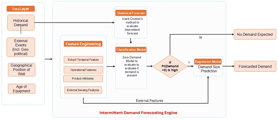
(Charts and figures courtesy of Jamalya Deb, MBA, MS)

This formulation builds upon Croston’s method as a foundation. D_t is demand at time t, with many periods of D_t equaling 0. The size on non-zero demand is represented by Z_t, and P_t captures the interval between non-zero demand and two instances of non-zero demand. The Croston’s metric evaluates the forecast as:

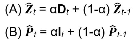
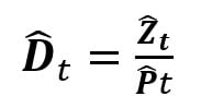
In the above, I_t is the time since the last non-zero demand and α is the smoothing factor ∈ (0 or 1). Using equations (A) and (B), demand forecast at time t can be computed using this equation:

However, as Croston’s method does not covariate and assumes stationary data, we must utilize the projection to develop a classification model to further re-enforce the decision and model:

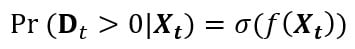
In this equation, X_t is the feature set created with Croston’s projection D_t as one of the features, along with internal and external factors, and σ is sigmoid function. Also, f represents the classifier used for modelling.

In our case, we used the XGBoost model as a classifier. The classification model helps to identify if there is a demand expected. If the Pr (D_t > o| X_t) > threshold, then the regression model is executed to evaluate the expected demand size:

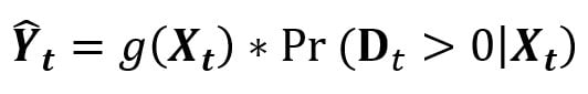
In the above equation, g(.) is the regression function and Y_t  is the expected demand adjusted for probability Pr (D_t > o| X_t). The current method also utilizes the XGBoost model as the regressor.  

Utilizing this method, we achieved significant experimentation results and observed valuable learnings. We used mean absolute percentage error (MAPE) for evaluation of model performance by the following:

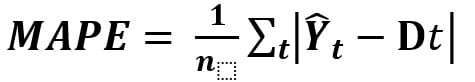
Here, Z is the set of non-zero demand periods.

Compiling the Results

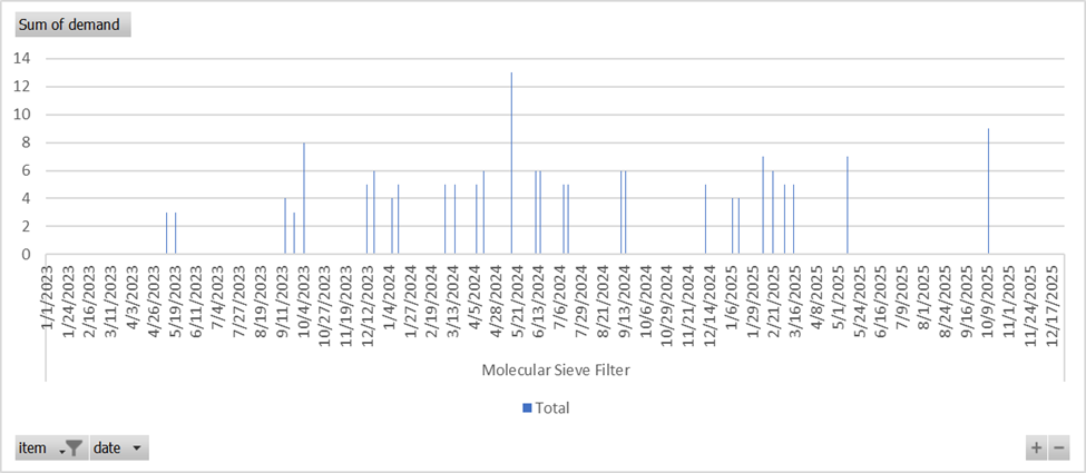
The hybrid method has been applied to three years’ worth of data with day level resolution. Illustrative data is shown for five part numbers with variable levels of intermittency.  The average demand interval is close to 25 days with a coefficient of variation (COV) of 0.26. Demand distribution is shown in Figures 1-4 at the bottom.

The hybrid method has been applied to the above series and benchmarked against traditional methods, as shown in the table below.

Further, temporal aggregation has been applied to the hybrid method at different resolution of time aggregations, as noted in Figure 5 at the bottom. In this aggregation, we observed the following outcomes:

• Discrete ARIMA: poor with zero-heavy series, sensitive to data sparsity
• INARMA: accurate for count data, rarely available in Python; complex fitting
• Croston: simple, popular for ADI greater than 20
• Adjusted Croston: more accurate than Croston on low COV
• Hybrid method: used to improve interval forecasts, depends on base model.

Based on the above performance, the base Croston method has been utilized to extract intermittency patterns from the series, followed by a classification-based method to predict whether there is demand or not in the next time horizon. The probability of whether the regression model has to be triggered has been optimized via running simulations that minimize the MAPE probability with a threshold set to 0.76.

Utilizing this hybrid method, businesses have reported that dynamic adjustment of reorder points has shown on-time delivery improvement in the range of 10 percent to 14 percent. Procurement teams have reported (1) a 25 percent to 30 percent reduction in manual expediting activities and (2) a reduction in stockouts by as much as 20 percent to 22 percent.  These reductions have generated significant uplift in supply chain team morale, as well as improvements in cross-functional collaboration.

Making a Forecasting Difference

By leveraging the hybrid forecasting method, manufacturers and distributors can achieve optimized inventory management, striking an effective balance that minimizes average on-hand stock levels.

This approach thus reduces costs associated with excess inventory while freeing up valuable working capital. By adopting this methodology, businesses can establish dynamic reorder points, driven by forecasted lead-time demand, which seamlessly integrate with MRP systems to align supply with demand. This shift empowers factory operations to adopt a proactive strategy, moving away from reactive measures and enhancing operational agility.

With diminished demand uncertainty, suppliers benefit from reduced stockout incidents and gain deeper insights into customer requirements. This enhanced visibility, coupled with timely engagement, fosters stronger supplier-customer relationships, paving the way for increased business opportunities.

The most significant impact, however, lies in the substantial cost savings for manufacturers. By precisely aligning raw material procurement with service-level demands and fine-tuning production capacity to match output needs, manufacturers can achieve peak productivity and operational excellence.

Furthermore, refining the hybrid forecasting model has the potential to be a game-changer for supply chains, enabling unprecedented accuracy in demand prediction, streamlining operations, and positioning organizations at the forefront of industry innovation.

Intermittent Demand Distribution, Parts A-E

Figure 1

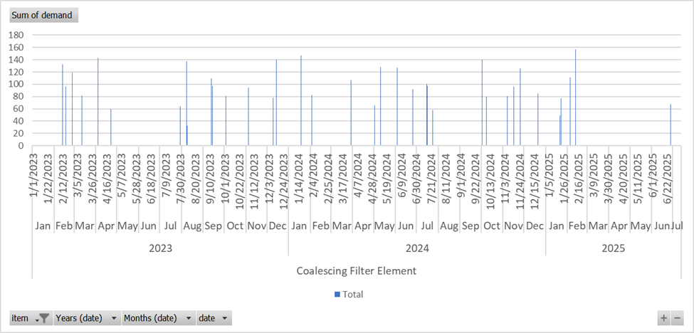
Figure 2

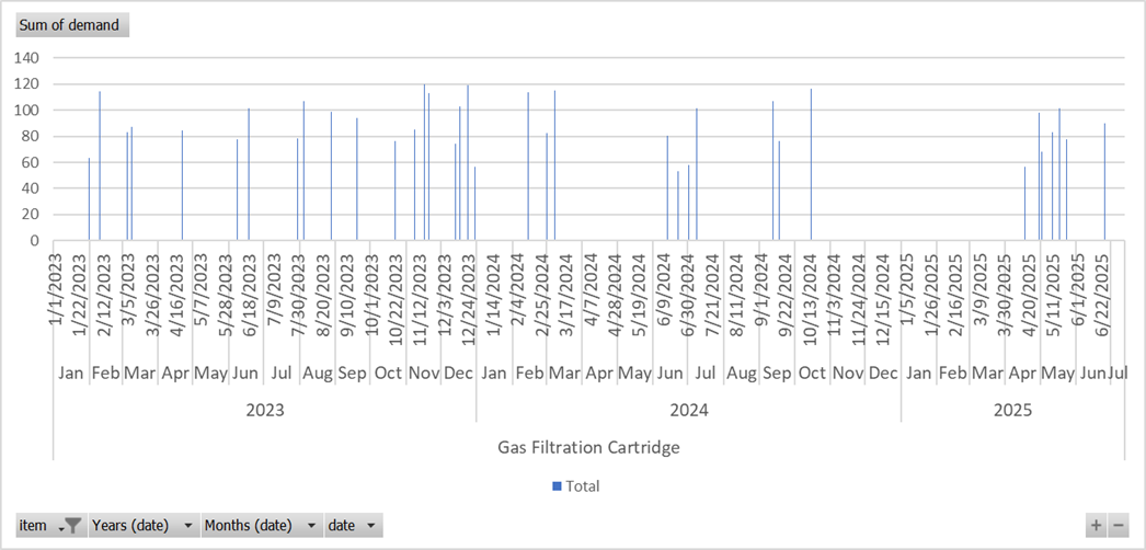
Figure 3

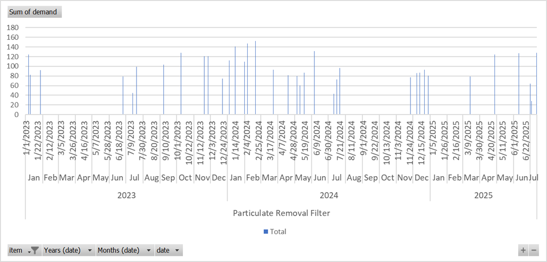
Figure 4

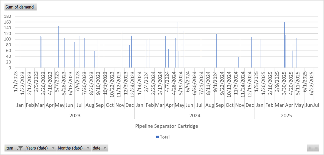
Figure 5

(Top photo credit: Getty Images/Eclipse Images)