How Many Stations Are Needed For 30-Minute Delivery?

Editor’s note: This is the second of a two-part series on selecting distribution center locations. The first article can be read here.

***

Let’s say that an e-commerce retailer specializing in ultra-fast delivery promises customers delivery within one hour of ordering for a selected assortment of products. Budgeting 30 minutes for picking and packing orders, that means last-mile delivery stations need to be within 30 minutes’ driving distance of customers.

How many last-mile delivery stations are needed in a metro area, and approximately where should they be?

Circuity Factors

In the first article, we used circuity factors to get a quick pulse on the number of distribution centers (DCs) and their approximate locations that are necessary nationally to meet a service goal of reaching 95 percent of demand within a one-day drive of a DC.

Circuity factors are a convenient rule-of-thumb that allows us to convert “as the crow flies” straight-line distance to an estimated driving distance by adding on an additional percentage (15 percent is common). For example, a 300-mile straight-line distance can be estimated at 300 multiplied by 115 percent, calculated to 345 driving miles. You can divide that driving miles estimate by a speed planning factor (in miles or kilometers per hour) to estimate drive time.

Circuity factors are great for national-level DC planning. But they tend to be less useful at more local levels, where real-life circuity factors and speed may be quite different.

For example, compare two short trips in the same suburb of Minneapolis. In both trips, the origin and destination are, as the crow flies, 2 miles apart.

• In the first trip, both origin and destination are just off a high-speed, straight thoroughfare. The driving distance is 2.1 miles. In this case, the circuity factor will be a very low 5 percent (2.1 divided by two, then minus one, which equals .05 ).
• In the second trip, both origin and destination are at the end of a complex set of cul-de-sacs and side streets, separated by a large lake. (Minnesota, after all, is the land of ) The driving distance is 2.7 miles. In this case, the circuity factor is a very high 35 percent (2.7 divided by 2, then minus 1, which equals .35 ).

While both trips are in the same city and the same straight-line distance, you wouldn’t use the common 15-percent circuity factor in your planning. It gets even more complex when you consider that shorter trips tend to have higher circuity factors than longer trips, even within the same city. Circuity factors can also be radically different between metro areas and between urban cores, suburban areas and rural areas.

So, while circuity factors are great for national-level DC modeling, they fail at shorter distances. Something else is needed.

Mapping Fast and Hyperlocal Delivery

For the fast and hyperlocal example, let’s look at other factors. Let’s say the delivery area is the Minneapolis-St. Paul metropolitan area. We can first look at census tracts, which are smaller than ZIP codes. In the seven-county Minneapolis-St. Paul area, there are 784 census tracts; the below map depicts their boundaries, which are colored by population.

A good starting assumption is to treat each census tract as a customer demand point and assume each census tract’s demand is proportional to its population. However, it’s best to use machine learning models to predict SKU-level customer demand at a hyperlocal level. This is one way that machine learning and optimization modeling are used together to make optimal supply chain decisions.

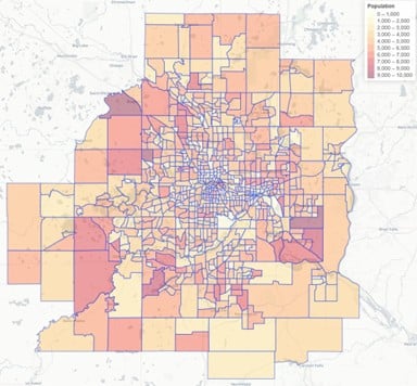
(Maps courtesy of Data Driven Supply Chain LLC)

To model potential last-mile delivery station locations, we will use 153 ZIP codes across the Minneapolis-St. Paul metro area. We could also go more detailed, using all 754 census tracts as potential delivery station locations. Or, if we already have potential commercial real estate sites identified, we can use them instead of ZIP codes.

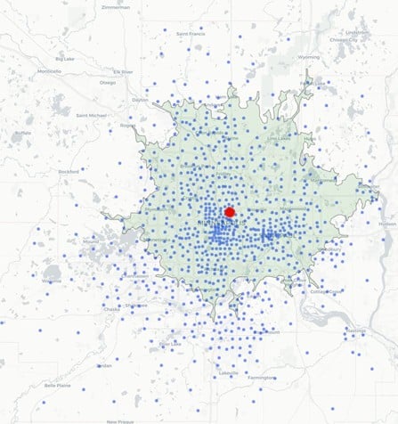
For each of the 153 ZIP codes, we will identify the area that can be reached within a 30-minute drive. For example, if we set up a delivery station in Northeast Minneapolis (the red dot in the below map, located in ZIP code 55413), the 30-minute delivery zone is the light green area. Each blue dot represents a demand point, using the census tract.

Thus, the map shows that 62 percent of the metro population is within a 30-minute drive of this delivery station.

We can build 30-minute delivery zones for every one of the ZIP codes we are considering for last-mile delivery stations. For each of these ZIP codes, we can then calculate which demand points are within the 30-minute delivery zone. Then, using optimization modeling, the math underlying supply chain design software, we can identify the smallest number of delivery stations and their locations that will enable us to cover 95 percent of the metro population within a 30-minute delivery zone.

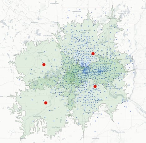
The model suggests that four delivery stations are needed to meet this goal. They are located near the suburban “corners” of the metro area. Some demand points are within the 30-minute delivery zones of multiple delivery stations. The next map depicts the color differences from lightest to darkest greens. The blue dots outside the green background represent the 5 percent of demand that is not within a 30-minute drive of any delivery station.

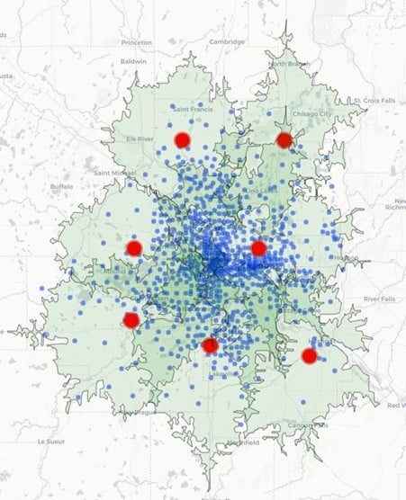
If we have a higher service level goal — say, 99 percent of the population within a 30-minute drive of a delivery station — seven delivery stations are needed, as shown in the last map.

If your business depends upon fast, hyperlocal delivery, proper location of your delivery stations is critical. In addition to delivery zones as seen in this article, you should layer in operational considerations of multi-stop routing and building capacity.

As a first step, using a combination of census tracts, machine learning, and optimization can help identify optimal delivery station locations to meet your hyperlocal coverage goal.